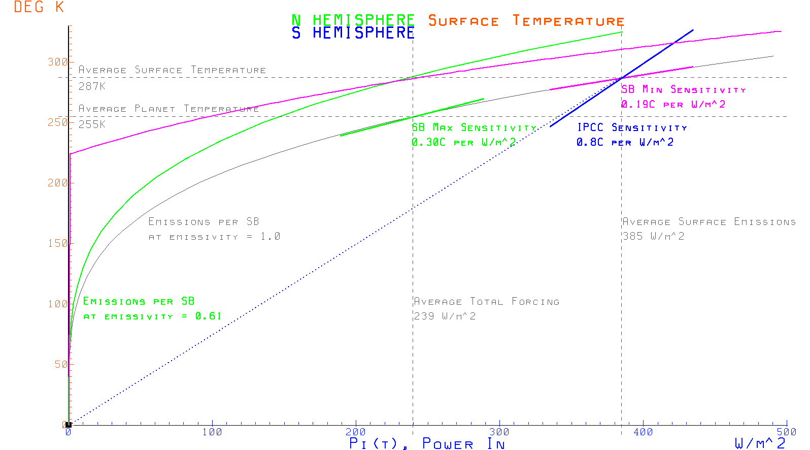
This first plot shows the predictions of the simplified model. The green line is the prediction of the LTE relationship between the surface temperature (Y axis) and the power emitted by the planet (X axis). The magenta line is the prediction of the LTE relationship between the surface temperature (Y axis) and the solar power arriving at the planet, after reflection (X axis). The prediction of the output relationship is the Stefan-Boltzmann Law quantifying a gray body whose emissivity is 0.61. The magenta line is the Stefan-Boltzmann Law for an ideal black body whose temperature is the same as the surface, except that it is biased up to the operating point of the system. Where these two predictions intersect defines the operating point corresponding to the planets average behavior, where the dynamic behavior is centered around this point. The gray line is for reference and shows the Stefan-Boltzmann Law describing an ideal black body (emissivity = 1). Along this relationship short green and magenta lines are shown to represent the sensitivites of the input and output path at the operating point of the planet. Shown in blue and drawn to the same scale as the predictions is a representation of the sensitivity claimed by the IPCC.
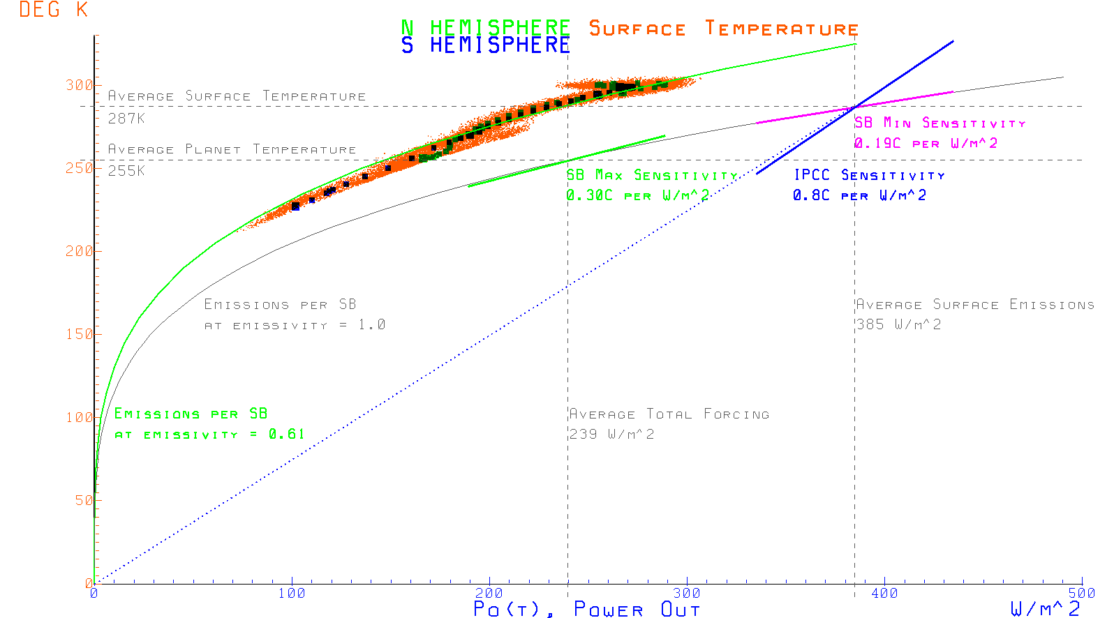
This next plot shows how the measurements correspond to the prediction of the relationship between the surface temperature and the planets emissions as a scatted plot. The small orange dots are the monthly averages for each 2.5 degree slice of the planet. The larger dots are the averages for each slice across nearly 3 deacades of monthly. Northern hemisphere slice averages are the larger green dots and Southern hemisphere slices are the larger blue dots. The colors are hard to discern since the S hemisphere averages mostly align with the N hemisphere averages and making the larger dots appear black. Even the monthly average align relatively closely with the prediction while the multi-year averages align almost exactly.
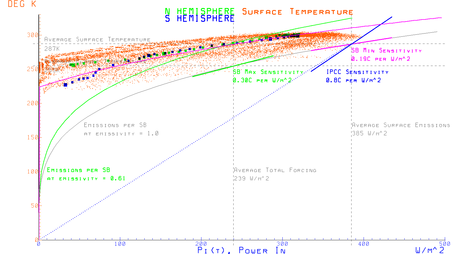
This next plot shows the measured relationship between the surface temperature and incident power from the Sun. Again, the small dots are monthly averages while the larger dots are the average over the whole data set. While the monthly averages show more deviation from the prediction, the long term LTE averages coincide almost exactly. The deviation of the monthly averages is expected as the incident power varies faster than the planet can respond to them. The sensitivity is delta Y (the change in temperature) divided by delta X (the change in input power) at the average temperature. This is about 0.19 C per W/m^2. Note that the sensitivity of the output path, calculated in the same manner is about 0.3C per W/m^2. The average sensitivty of the planet will be somewhere between these two limits.
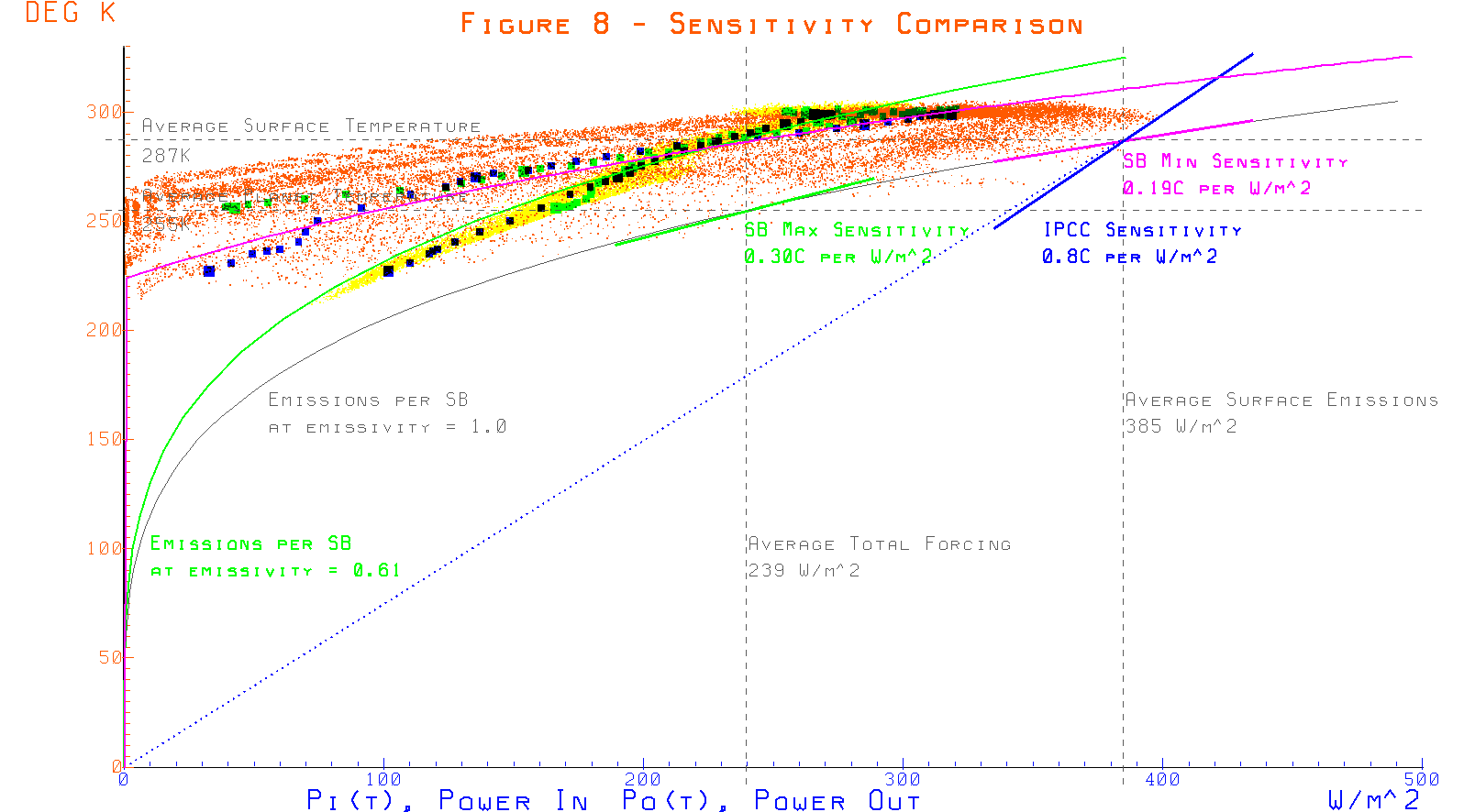
This last plot combines the above layers where the output relationship is yellow to differentiate it from the input relationship.